![]()
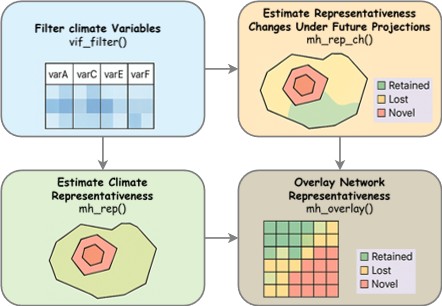
The ClimaRep package offers tools to analyze the climate
representativeness of defined areas, assessing current conditions and
evaluating how they are projected to change under future scenarios.
Using spatial data, including climate raster layers, the input reference
area polygons, and a polygon of the study area, the package quantifies
this representativeness and analyzes its transformation.
Key features include: * Filtering raster climate variables to reduce
multicollinearity (ClimaRep::vif_filter()). * Estimating
current climate representativeness (ClimaRep::mh_rep()). *
Estimating changes in climate representativeness under future climate
projections (ClimaRep::mh_rep_ch()). * Estimating climate
representativeness overlay (ClimaRep::rep_overlay()).
You can install the development version of ClimaRep from
CRAN with:
install.packages("ClimaRep")Alternatively, you can install the development version from GitHub:
install.packages("devtools")
library(devtools)
devtools::install_github("MarioMingarro/ClimaRep")
Dependencies:
This package relies on other R packages, such as:
terrafor efficient handling of raster data (SpatRasterobjects).
sffor robust handling of vector data (sfobjects).
statsfor statistical analysis.
ggplot2andtidyterrafor visualization tasks.
These dependencies will be installed automatically when you install
ClimaRep.
This section provides a brief example demonstrating the core workflow of the package.
First, load the package:
library(ClimaRep)
library(terra)
library(sf)
Next, prepare the essential input data:
Climate variables as an SpatRaster
objects with consistent extent, resolution, and Coordinate Reference
System (CRS).
Polygon as an sf object containing
one or more polygons, with a column identifying each reference area
(e.g., a ‘name’ or ‘ID’ column).
Study area as a single sf object,
representing the overall geographical region for analysis and thus the
climate space being worked on.
Here is a practical example using simulated data:
The example simulates a pair of reference polygon and
assesses their climate representativeness and change, based on
Mahalanobis Distance.
This involves creating a simulated climate space within which the analysis is performed.
Generate simulated climate raster layers:
set.seed(2458)
n_cells <- 100 * 100
r_clim_present <- terra::rast(ncols = 100, nrows = 100, nlyrs = 7)
values(r_clim_present) <- c(
  (rowFromCell(r_clim_present, 1:n_cells) * 0.2 + rnorm(n_cells, 0, 3)),
  (rowFromCell(r_clim_present, 1:n_cells) * 0.9 + rnorm(n_cells, 0, 0.2)),
  (colFromCell(r_clim_present, 1:n_cells) * 0.15 + rnorm(n_cells, 0, 2.5)),
  (colFromCell(r_clim_present, 1:n_cells) +
     rowFromCell(r_clim_present, 1:n_cells) * 0.1 + rnorm(n_cells, 0, 4)),
  (colFromCell(r_clim_present, 1:n_cells) /
     rowFromCell(r_clim_present, 1:n_cells) * 0.1 + rnorm(n_cells, 0, 4)),
  (colFromCell(r_clim_present, 1:n_cells) *
     (rowFromCell(r_clim_present, 1:n_cells) + 0.1 + rnorm(n_cells, 0, 4))),
  (colFromCell(r_clim_present, 1:n_cells) *
     (colFromCell(r_clim_present, 1:n_cells) + 0.1 + rnorm(n_cells, 0, 4))))
names(r_clim_present) <- c("varA", "varB", "varC", "varD", "varE", "varF", "varG")
terra::crs(r_clim_present) <- "EPSG:4326"
terra::plot(r_clim_present)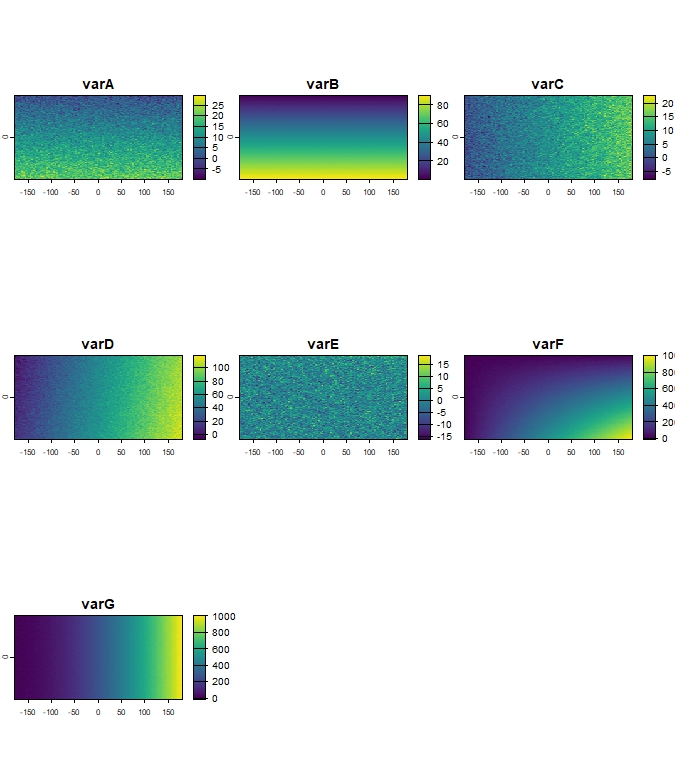
Figure 1: Example of simulated climate raster layers
(r_clim_present).
Multicollinearity among climate variables can affect multivariate analyses.
To handle this, the ClimaRep::vif_filter() function can
be used to iteratively remove variables with a Variance Inflation Factor
(VIF) above a specified threshold (e.g., th = 5).
The output returns a list object with: - A filtered
SpatRaster object containing only the variables that were
kept - A comprehensive statistics summary list including: -
The name of variables that were kept and those that were excluded. - The
original Pearson’s correlation matrix between all initial variables. -
The final VIF values for the variables that were retained.
vif_result <- vif_filter(r_clim_present, th = 5)
print(vif_result$summary)

Kept layers: varA, varC, varE, varF, varG
Excluded layers: varD, varB

Pearson correlation matrix of original data:
        varA    varB   varC   varD    varE    varF   varG
varA  1.0000  0.8870 0.0087 0.0938 -0.0745  0.5816 0.0028
varB  0.8870  1.0000 0.0043 0.0997 -0.0769  0.6513 0.0003
varC  0.0087  0.0043 1.0000 0.8523  0.0517  0.5676 0.8341
varD  0.0938  0.0997 0.8523 1.0000  0.0576  0.7077 0.9529
varE -0.0745 -0.0769 0.0517 0.0576  1.0000 -0.0256 0.0653
varF  0.5816  0.6513 0.5676 0.7077 -0.0256  1.0000 0.6305
varG  0.0028  0.0003 0.8341 0.9529  0.0653  0.6305 1.0000

Final VIF values for kept variables:
        VIF
varA 2.2832
varC 3.3473
varE 1.0121
varF 3.8325
varG 4.3545

r_clim_present_filtered <- vif_result$filtered_raster
terra::plot(r_clim_present_filtered)
Figure 2: Example of filtered climate dataset, showing remaining
variables (r_clim_present_filtered) after
ClimaRep::vif_filter().
Create example reference polygon (sf) to
estimate climate representativeness and a study_area
polygon (sf) to set the climate space for analysis:
hex_grid <- sf::st_sf(
  sf::st_make_grid(
    sf::st_as_sf(
      terra::as.polygons(
        terra::ext(r_clim_present))),
  square = FALSE))
sf::st_crs(hex_grid) <- "EPSG:4326"
polygons <- hex_grid[sample(nrow(hex_grid), 2), ]
polygons$name <- c("Pol_1", "Pol_2")
sf::st_crs(polygons) <- sf::st_crs(hex_grid)
study_area_polygon <- sf::st_as_sf(as.polygons(terra::ext(r_clim_present)))
sf::st_crs(study_area_polygon) <- "EPSG:4326"
terra::plot(r_clim_present[[1]])
terra::plot(polygons, add = TRUE, color= "transparent", lwd = 3)
terra::plot(study_area_polygon, add = TRUE, col = "transparent", lwd = 3, border = "red")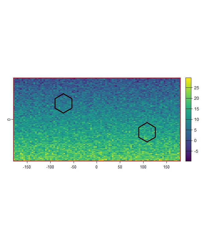
Figure 3: Example of reference polygons (black outline) and study
area (red outline) overlaid on
r_clim_present_filtered[[1]].
Use ClimaRep::mh_rep() to estimate climate
representativeness for each reference polygon.
The function calculates the Mahalanobis Distance from the
multivariate centroid of climate conditions within each reference
polygon to all cells in the study_area.
Cells within a certain percentile threshold (th) of
distances found within the reference polygon are considered
representative of the climate of the polygon.
mh_rep(
  polygon = polygons,
  col_name = "name",
  climate_variables = r_clim_present_filtered,
  study_area = study_area_polygon,
  th = 0.95,
  dir_output = tempdir(),
  save_raw = TRUE)

----------------------------
Validating and adjusting Coordinate Reference Systems (CRS)
Starting per-polygon processing:

Processing polygon: pol_1 (1 of 2)

Processing polygon: pol_1 (2 of 2)

All processes were completed

Output files in: C:\Users\AppData\Local\Temp\RtmpY1rKKD
----------------------------
This process generates 3 subfolders within the directory specified by
dir_output (e.g., tempdir()).
list.files(tempdir())
[1] "Charts" "Mh_Raw" "Representativeness"Charts subfolder contains the binary
representativeness image files (.jpeg) for each reference
polygon.list.files(file.path(tempdir(), "Charts"))
[1] "pol_1_rep.jpeg" "pol_2_rep.jpeg"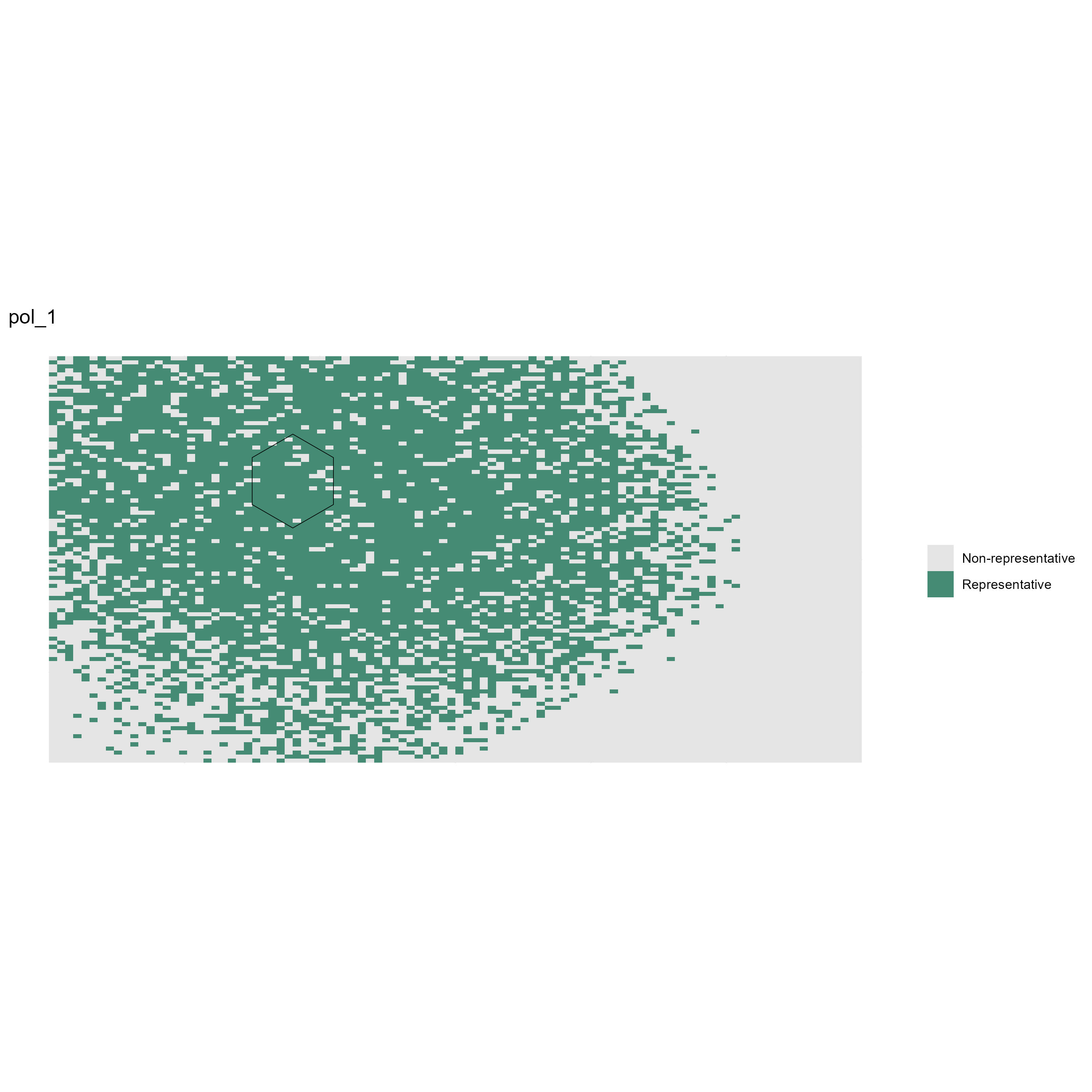
Figure 4: Example of binary representativeness map for Pol_1 (pol_1_rep.jpeg).
Mh_raw subfolder contains the continuous
Mahalanobis Distance rasters (.tif) for each reference
polygon.Lower values indicate climates more similar to the reference polygon’s centroid.
mh_rep_raw <- terra::rast(list.files(file.path(tempdir(), "Mh_Raw"),  pattern = "\\.tif$", full.names = TRUE))
terra::plot(mh_rep_raw[[1]])
terra::plot(polygons[1,], add = TRUE, color= "transparent", lwd = 3)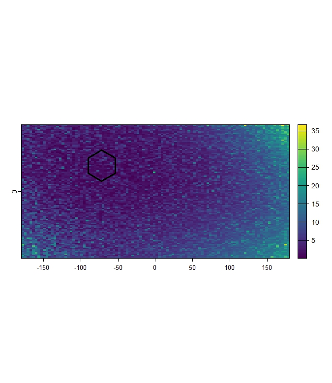
Figure 5: Example of continuous Mahalanobis Distance raster for Pol_1. Darker shades indicate cells with climate conditions more similar to Pol_1.
Representativeness subfolder contains the binary
representativeness rasters (.tif) for each reference
polygon, based on the threshold (th) applied
to the raw Mahalanobis Distance.Cells are coded 1 for Representative and
0 for Unsuitable.
mh_rep_result <- terra::rast(list.files(file.path(tempdir(), "Representativeness"),  pattern = "\\.tif$", full.names = TRUE))
terra::plot(mh_rep_result[[1]])
terra::plot(polygons[1,], add = TRUE, color= "transparent", lwd = 3)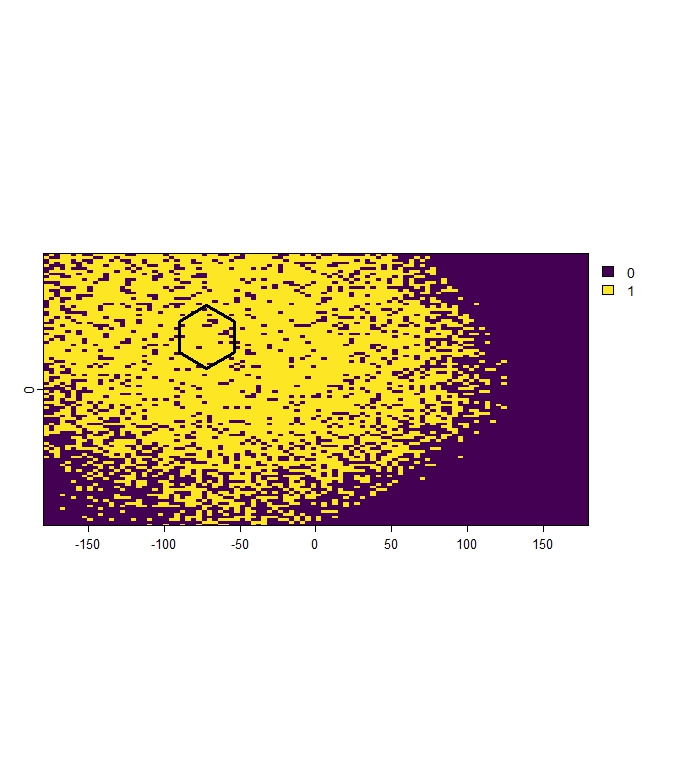
Figure 6: Example of binary representativeness raster for Pol_1, showing cells classified as representetive (value 1).
To estimate how representativeness changes, a future climate scenario is required.
In this example, a simple virtual future climate conditions
(SpatRaster) are created by adding a constant value to the
r_clim_present_filtered data:
r_clim_future <- r_clim_present_filtered + 2
names(r_clim_future) <- names(r_clim_present_filtered)
terra::crs(r_clim_future) <- terra::crs(r_clim_present_filtered)
terra::plot(r_clim_future)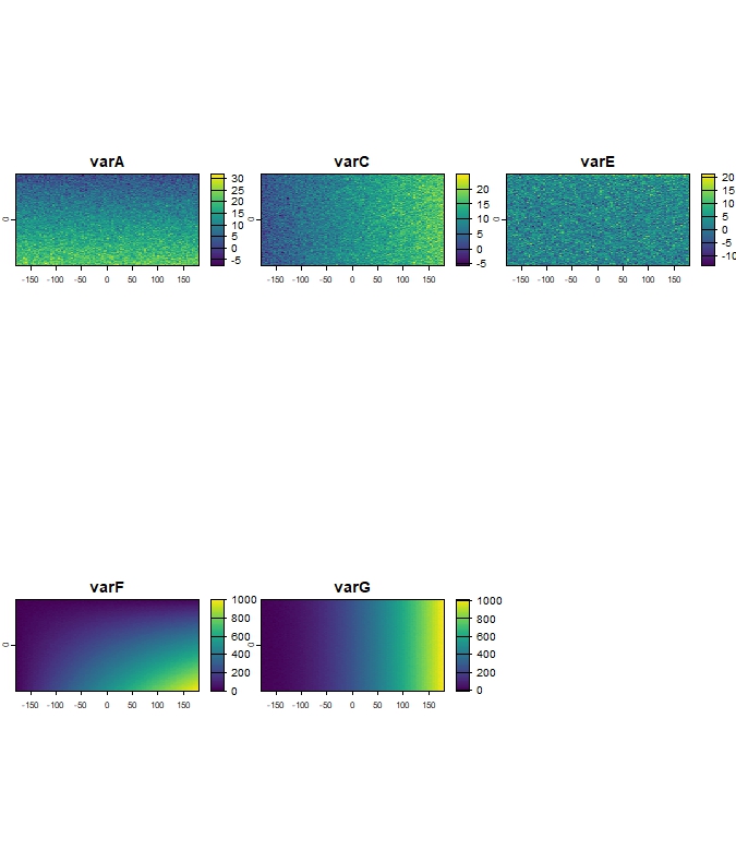
Figure 7: Example of simulated future climate variables
(r_clim_future).
Use ClimaRep::mh_rep_ch() to compare representativeness
of a reference polygon, between the
present_climate_variables and
future_climate_variables.
This function calculates representativeness for each reference
polygon in both scenarios and determines cells where
conditions:
mh_rep_ch(
polygon = polygons,
col_name = "name",
present_climate_variables = r_clim_present_filtered,
future_climate_variables = r_clim_future,
study_area = study_area_polygon,
th = 0.95,
model = "MODEL",
year = "2070",
dir_output = tempdir(),
save_raw = TRUE)

Validating and adjusting Coordinate Reference Systems (CRS).
Starting per-polygon processing:

Processing polygon: pol_1 (1 of 2)

Processing polygon: pol_2 (2 of 2)

All processes were completed

Output files in:  C:\Users\AppData\Local\Temp\RtmpY1rKKD
This process generates several subfolders within the directory
specified by dir_output.
list.files(tempdir())
 [1] "Change"             "Charts"             "Mh_Raw_Pre"             "Mh_Raw_Fut"
The Change subfolder contains binary rasters
(.tif) for each reference polygon, indicating
the category of change.
change_result <- terra::rast(list.files(file.path(tempdir(), "Change"),  pattern = "\\.tif$", full.names = TRUE))
terra::plot(change_result[[2]])
terra::plot(polygons[2,], add = TRUE, color= "transparent", lwd = 3)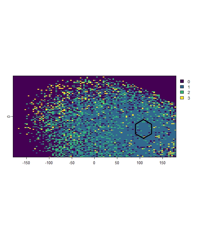
Figure 8: Example of change in representativeness for Pol_2, showing areas Unsuitable (0), Stable (1), Lost (2), Novel (3).
The Charts subfolder is updated or regenerated and
contains summary map files (.jpeg) visualizing the change
analysis results for each reference polygon.
list.files(file.path(tempdir(), "Charts"))
[1] "pol_1_rep_change.jpeg" "pol_2_rep_change.jpeg"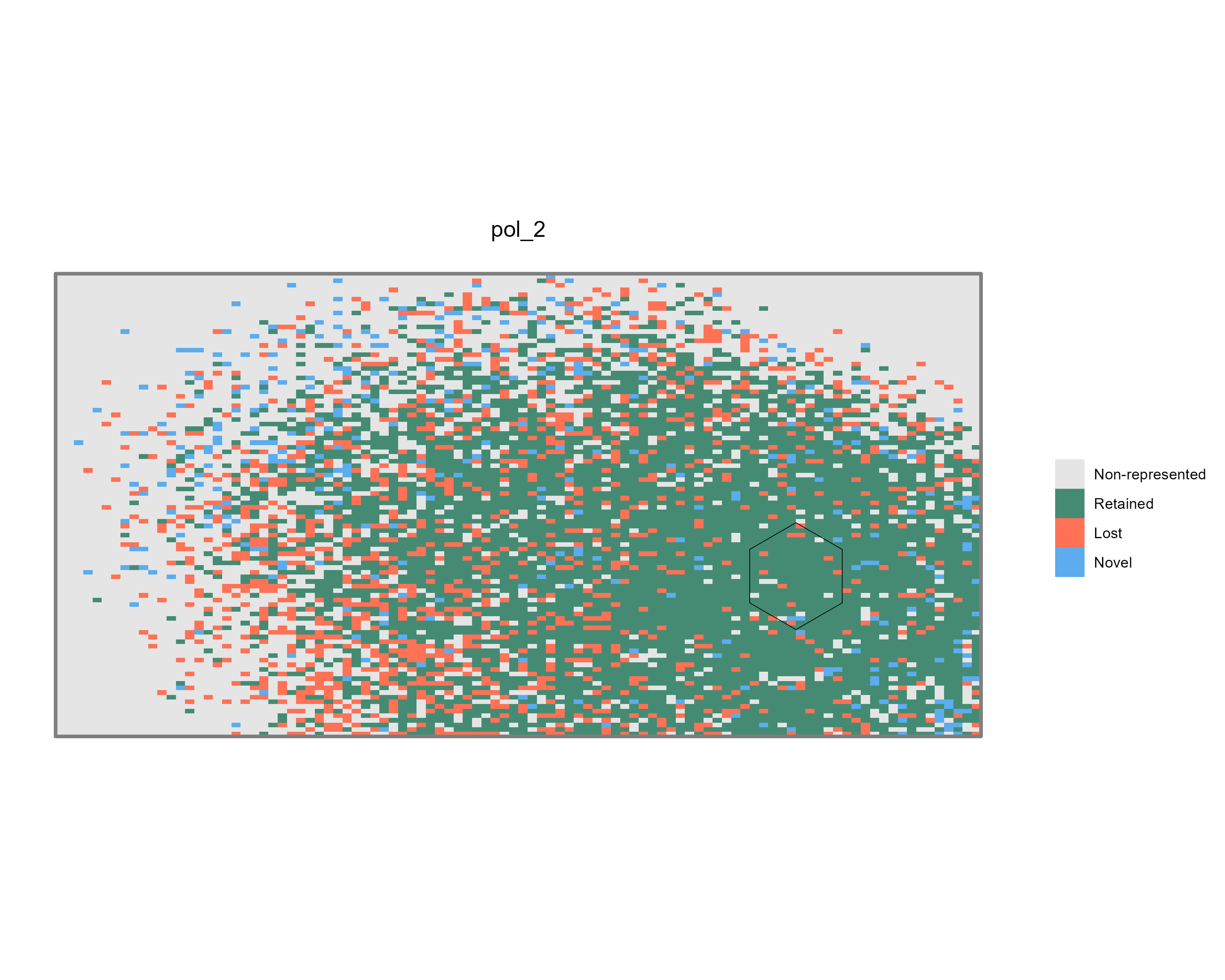
Figure 9: Example of summary maps illustrating climate
representativeness change for Pol_2
(pol_2_rep_change.jpeg).
The Mh_Raw_Pre subfolder contains the continuous
Mahalanobis Distance rasters (.tif) for the
present scenario, calculated within the
study_area extent relative to the climate conditions within
each reference polygon.
Mh_raw_Pre_result <- terra::rast(list.files(file.path(tempdir(), "Mh_Raw_Pre"),  pattern = "\\.tif$", full.names = TRUE))
terra::plot(Mh_raw_Pre_result[[2]])
terra::plot(polygons[2,], add = TRUE, color= "transparent", lwd = 3)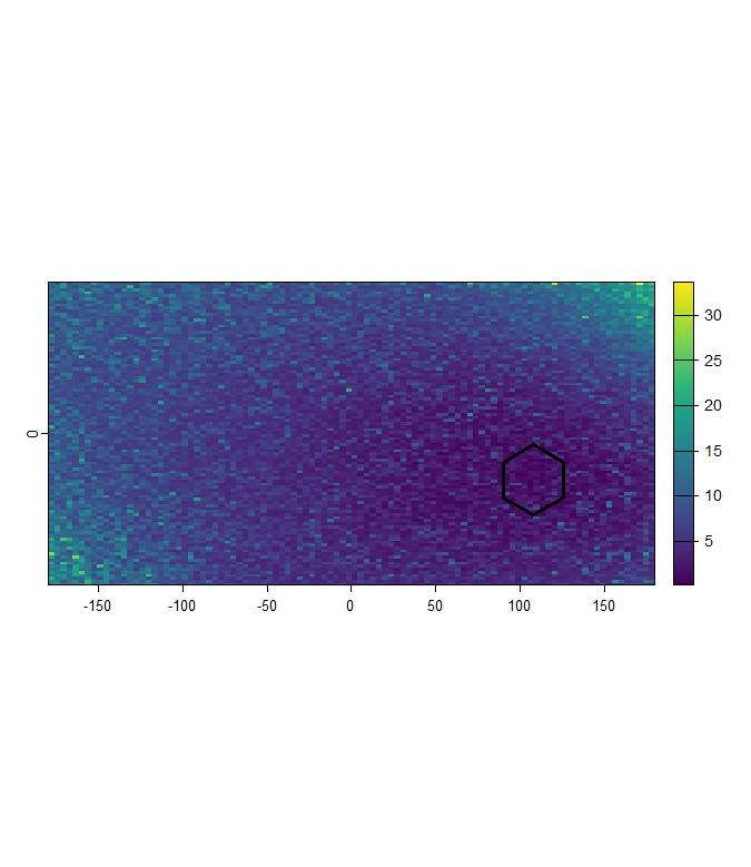
Figure 10: Example continuous present Mahalanobis Distance raster (within study area) for Pol_2.
The Mh_Raw_Fut subfolder contains the continuous raw
Mahalanobis Distance rasters (.tif) for the
future scenario, calculated within the
study_area extent relative to the climate conditions within
each reference polygon.
Mh_raw_Fut_result <- terra::rast(list.files(file.path(tempdir(), "Mh_Raw_Fut"),  pattern = "\\.tif$", full.names = TRUE))
terra::plot(Mh_raw_Fut_result[[2]])
terra::plot(polygons[2,], add = TRUE, color= "transparent", lwd = 3)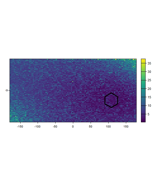
Figure 11: Example continuous future Mahalanobis Distance raster for Pol_2.
After obtaining the representativeness
(ClimaRep::mh_rep()), or change
(ClimaRep::mh_rep_ch()), rasters for multiple reference
polygons, it is possible to combine them and to identify
where the different types of changes (representative/stable, lost,
novel) are accumulated.
The ClimaRep::rep_overlay() function counting, for each
cell, how many of the input rasters had a specific category value at
that location.
ClimaRep_overlay <- rep_overlay(folder_path = file.path(tempdir(), "Change"),
                               output_dir = file.path(tempdir(), "ClimaRep_overlay"))

Processing 2 classification rasters from C:\Users\AppData\Local\Temp\RtmpY1rKKD/Change
Calculating counts for category: Lost (value = 2)
Calculating counts for category: Stable (value = 1)
Calculating counts for category: Novel (value = 3)
All processes were completed
Output files saved in:  C:\Users\AppData\Local\Temp\RtmpY1rKKD/ClimaRep_overlay

terra::plotRGB(ClimaRep_overlay, stretch = "lin")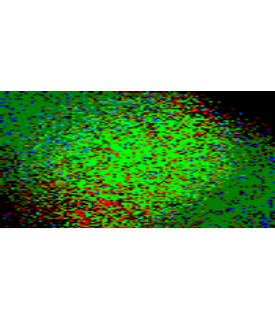
Figure 12: Visualisation of accumulated Lost (R), Stable (G) and
Novel (B) cells for both reference polygon.
terra::plot(ClimaRep_overlay)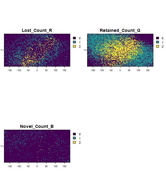
Figure 13: Example of accumulate Lost (1), Stable (2) or Novel
(3) cells for both reference polygon.
ClimaRep::vif_filter()
This function iteratively filters layers from a
SpatRaster object by removing the one with the highest
Variance Inflation Factor (VIF) that exceeds a specified threshold
(th).
ClimaRep::vif_filter(x, th)
x: ASpatRasterobject with climate layers.
th: The VIFthreshold.
ClimaRep::mh_rep()
This function calculates climate representativeness for each reference polygon within a defined area.
Representativeness is assessed by comparing the multivariate climate
conditions of each cell, of the reference climate space
(climate_variables), with the climate conditions within
each specific reference polygon. The CRS of
polygon will be used as the reference system.
ClimaRep::mh_rep(polygon, col_name, climate_variables, th, dir_output, save_raw)
polygon: Ansfobject containing the input polygon(s) for which representativeness will be assessed.
col_name: Thenameof the column inpolygonthat contains unique identifiers for each referencepolygon.
climate_variables: ASpatRasterobject with the climate layers (pre-filtered usingvif_filter).
study_area: Ansfobject defining the overall study region.
th: Thethresholdfor determining representativeness (e.g., 0.9 for the 90th percentile of distances within the referencepolygon).
dir_output: Path to thedirectorywhere output rasters and charts will be saved. The directory will be created if it doesn’t exist.
save_raw: Logical. IfTRUE, saves the continuous Mahalanobis Distance raster (Mh_raw) for each referencepolygon.
ClimaRep::mh_rep_ch()
This function calculates climate representativeness for each reference polygon across two time periods (present and future) within a defined area.
The function identifies areas of climate representativeness Stable, Lost, or Novel.
Representativeness change is assessed by comparing the multivariate
climate conditions of each cell, of the reference climate space
(present_climate_variables and
future_climate_variables), with the climate conditions
within each specific reference polygon. The CRS of
polygon will be used as the reference system.
ClimaRep::mh_rep_ch(polygon, col_name, present_climate_variables, future_climate_variables, study_area, th, model, year, dir_output, save_raw)
polygon: Ansfobject containing the input polygon/s for which representativeness change will be assessed.
col_name: Thenameof the column inpolygonthat contains unique identifiers for each referencepolygon.
present_climate_variables: ASpatRasterobject with the present climate layers (pre-filtered usingvif_filter).
future_climate_variables: ASpatRasterobject with the future climate layers (usually same aspresent_climate_variables).
study_area: Ansfobject defining the overall study region.
th: The percentilethresholdfor determining representativeness in both scenarios (e.g., 0.9 for the 90th percentile of distances within the referencepolygon).
model:Character stringidentifying the climate model (e.g., “MIROC6”). This is used in output filenames for clear identification.
year:Character stringidentifying the future period (e.g., “2050”). This is used in output filenames for clear identification.
dir_output: Path to thedirectorywhere output rasters and charts will be saved. The directory will be created if it doesn’t exist.
save_raw: Logical. IfTRUE, saves the continuous Mahalanobis Distance rasters (Mh_raw) for both present and future scenarios within the study area extent.
ClimaRep::rep_overlay()
Combines multiple single-layer rasters (tif), outputs
from ClimaRep::mh_rep() or
ClimaRep::mh_rep_ch() for different input polygons, into a
multi-layered SpatRaster.
This function handles inputs from both
ClimaRep::mh_rep() (which contains representetive and
unsuitable cells) and ClimaRep::mh_rep_ch() (which includes
Stable, Lost, and Novel cells). The output layers consistently represent
the accumulation of each input.
ClimaRep::rep_overlay(folder_path, dir_output)
folder_path:Character string. Path to the directory containing the input single-layer GeoTIFF classification rasters (outputs fromClimaRep::mh_rep_ch()orClimaRep::mh_rep()).dir_output: Path to thedirectorywhere output rasters will be saved. The directory will be created if it doesn’t exist.
If the package itself is formally cited (e.g., on CRAN), please include the package citation as well:
Mingarro & Lobo (2021) Connecting protected areas in the Iberian peninsula to facilitate climate change tracking. Environmental Conservation, 48(3): 182-191. doi:10.1017/S037689292100014X
Mingarro, Aguilera-Benavente & Lobo (2020) A methodology to assess the future connectivity of protected areas by combining climatic representativeness and land-cover change simulations: the case of the Guadarrama National Park (Madrid, Spain). Environmental Planning and Management, 64(4): 734–753. doi.org/10.1080/09640568.2020.1782859
Mingarro & Lobo (2018) Environmental representativeness and the role of emitter and recipient areas in the future trajectory of a protected area under climate change. Animal Biodiversity and Conservation, 41(2): 333–344. doi.org/10.32800/abc.2018.41.0333
Farber & Kadmon (2003) Assessment of alternative approaches for bioclimatic modeling with special emphasis on the Mahalanobis Distance. Ecological Modelling, 160: 115–130. doi:10.1016/S0304-3800(02)00327-7
If you encounter issues or have questions, please contact.
MIT, GPL-3