2017-11-11
Function “mytable”” produce table for descriptive analysis easily. It is most useful to make table to describe baseline characteristics common in medical research papers.
require(moonBook)
data(acs)
mytable(Dx~.,data=acs)
                 Descriptive Statistics by 'Dx'
_________________________________________________________________
                     NSTEMI       STEMI     Unstable Angina   p
                    (N=153)      (N=304)        (N=400)
-----------------------------------------------------------------
 age              64.3 ± 12.3  62.1 ± 12.1    63.8 ± 11.0   0.073
 sex                                                        0.012
   - Female        50 (32.7%)   84 (27.6%)    153 (38.2%)
   - Male         103 (67.3%)  220 (72.4%)    247 (61.8%)
 cardiogenicShock                                           0.000
   - No           149 (97.4%)  256 (84.2%)   400 (100.0%)
   - Yes           4 ( 2.6%)    48 (15.8%)     0 ( 0.0%)
 entry                                                      0.001
   - Femoral       58 (37.9%)  133 (43.8%)    121 (30.2%)
   - Radial        95 (62.1%)  171 (56.2%)    279 (69.8%)
 EF               55.0 ±  9.3  52.4 ±  9.5    59.2 ±  8.7   0.000
 height           163.3 ±  8.2 165.1 ±  8.2  161.7 ±  9.7   0.000
 weight           64.3 ± 10.2  65.7 ± 11.6    64.5 ± 11.6   0.361
 BMI              24.1 ±  3.2  24.0 ±  3.3    24.6 ±  3.4   0.064
 obesity                                                    0.186
   - No           106 (69.3%)  209 (68.8%)    252 (63.0%)
   - Yes           47 (30.7%)   95 (31.2%)    148 (37.0%)
 TC               193.7 ± 53.6 183.2 ± 43.4  183.5 ± 48.3   0.057
 LDLC             126.1 ± 44.7 116.7 ± 39.5  112.9 ± 40.4   0.004
 HDLC             38.9 ± 11.9  38.5 ± 11.0    37.8 ± 10.9   0.501
 TG               130.1 ± 88.5 106.5 ± 72.0  137.4 ± 101.6  0.000
 DM                                                         0.209
   - No            96 (62.7%)  208 (68.4%)    249 (62.2%)
   - Yes           57 (37.3%)   96 (31.6%)    151 (37.8%)
 HBP                                                        0.002
   - No            62 (40.5%)  150 (49.3%)    144 (36.0%)
   - Yes           91 (59.5%)  154 (50.7%)    256 (64.0%)
 smoking                                                    0.000
   - Ex-smoker     42 (27.5%)   66 (21.7%)    96 (24.0%)
   - Never         50 (32.7%)   97 (31.9%)    185 (46.2%)
   - Smoker        61 (39.9%)  141 (46.4%)    119 (29.8%)
-----------------------------------------------------------------
The first argument of function mytable is an object of
class formula. Left side of ~ must contain the name of one
grouping variable or two grouping variables in an additive
way(e.g. sex+group~), and the right side of ~ must have variables in an
additive way. . is allowed on the right side of formula
which means all variables in the data.frame specified by the 2nd
argument data. The sample data ‘acs’ containing demographic
data and laboratory data of 857 patients with acute coronary
syndrome(ACS). For more information about the data acs, type ?acs in
your R console.
str(acs)'data.frame': 857 obs. of 17 variables:
$ age : int 62 78 76 89 56 73 58 62 59 71 ...
$ sex : chr "Male" "Female" "Female" "Female" ...
$ cardiogenicShock: chr "No" "No" "Yes" "No" ...
$ entry : chr "Femoral" "Femoral" "Femoral" "Femoral" ...
$ Dx : chr "STEMI" "STEMI" "STEMI" "STEMI" ...
$ EF : num 18 18.4 20 21.8 21.8 22 24.7 26.6 28.5 31.1 ...
$ height : num 168 148 NA 165 162 153 167 160 152 168 ...
$ weight : num 72 48 NA 50 64 59 78 50 67 60 ...
$ BMI : num 25.5 21.9 NA 18.4 24.4 ...
$ obesity : chr "Yes" "No" "No" "No" ...
$ TC : num 215 NA NA 121 195 184 161 136 239 169 ...
$ LDLC : int 154 NA NA 73 151 112 91 88 161 88 ...
$ HDLC : int 35 NA NA 20 36 38 34 33 34 54 ...
$ TG : int 155 166 NA 89 63 137 196 30 118 141 ...
$ DM : chr "Yes" "No" "No" "No" ...
$ HBP : chr "No" "Yes" "Yes" "No" ...
$ smoking : chr "Smoker" "Never" "Never" "Never" ...You can choose the grouping variable(s) and row-variable(s) with the
formula.
mytable(sex~age+Dx,data=acs)
         Descriptive Statistics by 'sex'
__________________________________________________
                       Female       Male       p
                       (N=287)     (N=570)
--------------------------------------------------
 age                 68.7 ± 10.7 60.6 ± 11.2 0.000
 Dx                                          0.012
   - NSTEMI          50 (17.4%)  103 (18.1%)
   - STEMI           84 (29.3%)  220 (38.6%)
   - Unstable Angina 153 (53.3%) 247 (43.3%)
--------------------------------------------------
You can choose row-variable(s) with . and +
and - and variable name in an additive way.
mytable(am~.-hp-disp-cyl-carb-gear,data=mtcars)
   Descriptive Statistics by 'am'
____________________________________
            0           1        p
         (N=19)      (N=13)
------------------------------------
 mpg   17.1 ±  3.8 24.4 ±  6.2 0.000
 drat   3.3 ±  0.4  4.0 ±  0.4 0.000
 wt     3.8 ±  0.8  2.4 ±  0.6 0.000
 qsec  18.2 ±  1.8 17.4 ±  1.8 0.206
 vs                            0.556
   - 0 12 (63.2%)   6 (46.2%)
   - 1  7 (36.8%)   7 (53.8%)
------------------------------------ By default continuous variables are analyzed as normal-distributed
and are described with mean and standard deviation. To change default
options, you can use the method argument. Possible values
of method argument are:
When continuous variables are analyzed as non-normal, they are described with median and interquartile range.
mytable(sex~height+weight+BMI,data=acs,method=3)
           Descriptive Statistics by 'sex'
_____________________________________________________
              Female               Male           p
              (N=287)             (N=570)
-----------------------------------------------------
 height 155.0 [150.0;158.0] 168.0 [164.0;172.0] 0.000
 weight  58.0 [50.0;63.0]    68.0 [62.0;75.0]   0.000
 BMI     24.0 [22.1;26.2]    24.2 [22.2;26.2]   0.471
-----------------------------------------------------
Because the method argument is selected as 3, a
Shapiro-Wilk test normality test is used to decide if the variable is
normal or non-normal distributed. Note that height and
BMI was described as mean \(\pm\) sd, whereas the weight was described
as median and interquartile range.
In many cases, categorical variables are usually coded as numeric.
For example, many people usually code 0 and 1 instead of “No” and “Yes”.
Similarly, factor variables with three or four levels are coded 0/1/2 or
0/1/2/3. In many cases, if we analyze these variables as continuous
variables, we are not able to get the right result. In
mytable, variables with less than five unique
values are treated as a categorical variables.
mytable(am~.,data=mtcars)
    Descriptive Statistics by 'am'
_______________________________________
             0            1         p
          (N=19)        (N=13)
---------------------------------------
 mpg    17.1 ±  3.8  24.4 ±  6.2  0.000
 cyl                              0.013
   - 4   3 (15.8%)    8 (61.5%)
   - 6   4 (21.1%)    3 (23.1%)
   - 8  12 (63.2%)    2 (15.4%)
 disp  290.4 ± 110.2 143.5 ± 87.2 0.000
 hp    160.3 ± 53.9  126.8 ± 84.1 0.180
 drat    3.3 ±  0.4   4.0 ±  0.4  0.000
 wt      3.8 ±  0.8   2.4 ±  0.6  0.000
 qsec   18.2 ±  1.8  17.4 ±  1.8  0.206
 vs                               0.556
   - 0  12 (63.2%)    6 (46.2%)
   - 1   7 (36.8%)    7 (53.8%)
 gear                             0.000
   - 3  15 (78.9%)     0 ( 0.0%)
   - 4   4 (21.1%)    8 (61.5%)
   - 5   0 ( 0.0%)    5 (38.5%)
 carb    2.7 ±  1.1   2.9 ±  2.2  0.781
---------------------------------------
In mtcars data, all variables are expressed as numeric.
But as you can see, cyl, vs and
gear is treated as categorical variables. The
carb variables has six unique values and
treated as continuous variables. If you wanted the carb
variable to be treated as categorical variable, you can changed the
max.ylev argument.
mytable(am~carb,data=mtcars,max.ylev=6)
  Descriptive Statistics by 'am'
__________________________________
           0          1        p
         (N=19)     (N=13)
----------------------------------
 carb                        0.284
   - 1 3 (15.8%)  4 (30.8%)
   - 2 6 (31.6%)  4 (30.8%)
   - 3 3 (15.8%)   0 ( 0.0%)
   - 4 7 (36.8%)  3 (23.1%)
   - 6  0 ( 0.0%) 1 ( 7.7%)
   - 8  0 ( 0.0%) 1 ( 7.7%)
---------------------------------- If you wanted to make two separate tables and combine into one table,
mytable is the function of choice. For
example, if you wanted to build separate table for female and male
patients stratified by presence or absence of DM and combine it,
mytable(sex+DM~.,data=acs)
                 Descriptive Statistics stratified by 'sex' and 'DM'
_____________________________________________________________________________________
                                    Male                             Female
                     -------------------------------- -------------------------------
                          No           Yes        p        No          Yes        p
                       (N=380)       (N=190)           (N=173)      (N=114)
-------------------------------------------------------------------------------------
 age                 60.9 ± 11.5   60.1 ± 10.6  0.472 69.3 ± 11.4  67.8 ±  9.7  0.257
 cardiogenicShock                               0.685                           0.296
   - No              355 (93.4%)   175 (92.1%)        168 (97.1%)  107 (93.9%)
   - Yes              25 ( 6.6%)   15 ( 7.9%)          5 ( 2.9%)    7 ( 6.1%)
 entry                                          0.552                           0.665
   - Femoral         125 (32.9%)   68 (35.8%)          74 (42.8%)   45 (39.5%)
   - Radial          255 (67.1%)   122 (64.2%)         99 (57.2%)   69 (60.5%)
 Dx                                             0.219                           0.240
   - NSTEMI           71 (18.7%)   32 (16.8%)          25 (14.5%)   25 (21.9%)
   - STEMI           154 (40.5%)   66 (34.7%)          54 (31.2%)   30 (26.3%)
   - Unstable Angina 155 (40.8%)   92 (48.4%)          94 (54.3%)   59 (51.8%)
 EF                  56.5 ±  8.3   53.9 ± 11.0  0.007 56.0 ± 10.1  56.6 ± 10.0  0.655
 height              168.1 ±  5.8 167.5 ±  6.7  0.386 153.9 ±  6.5 153.6 ±  5.8 0.707
 weight              68.1 ± 10.4   69.8 ± 10.2  0.070 56.5 ±  8.7  58.4 ± 10.0  0.106
 BMI                 24.0 ±  3.1   24.9 ±  3.5  0.005 23.8 ±  3.2  24.8 ±  4.0  0.046
 obesity                                        0.027                           0.359
   - No              261 (68.7%)   112 (58.9%)        121 (69.9%)   73 (64.0%)
   - Yes             119 (31.3%)   78 (41.1%)          52 (30.1%)   41 (36.0%)
 TC                  184.1 ± 46.7 181.8 ± 44.5  0.572 186.0 ± 43.1 193.3 ± 60.8 0.274
 LDLC                117.9 ± 41.8 112.1 ± 39.4  0.115 116.3 ± 35.2 119.8 ± 48.6 0.519
 HDLC                38.4 ± 11.4   36.8 ±  9.6  0.083 39.2 ± 10.9  38.8 ± 12.2  0.821
 TG                  115.2 ± 72.2 153.4 ± 130.7 0.000 114.2 ± 82.4 128.4 ± 65.5 0.112
 HBP                                            0.000                           0.356
   - No              205 (53.9%)   68 (35.8%)          54 (31.2%)   29 (25.4%)
   - Yes             175 (46.1%)   122 (64.2%)        119 (68.8%)   85 (74.6%)
 smoking                                        0.386                           0.093
   - Ex-smoker       101 (26.6%)   54 (28.4%)          34 (19.7%)   15 (13.2%)
   - Never            77 (20.3%)   46 (24.2%)         118 (68.2%)   91 (79.8%)
   - Smoker          202 (53.2%)   90 (47.4%)          21 (12.1%)   8 ( 7.0%)
------------------------------------------------------------------------------------- If you want more beautiful table in your R markdown file, you can use myhtml function.
out=mytable(Dx~.,data=acs)
myhtml(out)| Dx |
NSTEMI (N=153) |
STEMI (N=304) |
Unstable Angina (N=400) |
p |
|---|---|---|---|---|
| age | 64.3 ± 12.3 | 62.1 ± 12.1 | 63.8 ± 11.0 | 0.073 |
| sex | 0.012 | |||
| Female | 50 (32.7%) | 84 (27.6%) | 153 (38.2%) | |
| Male | 103 (67.3%) | 220 (72.4%) | 247 (61.8%) | |
| cardiogenicShock | 0.000 | |||
| No | 149 (97.4%) | 256 (84.2%) | 400 (100.0%) | |
| Yes | 4 ( 2.6%) | 48 (15.8%) | 0 ( 0.0%) | |
| entry | 0.001 | |||
| Femoral | 58 (37.9%) | 133 (43.8%) | 121 (30.2%) | |
| Radial | 95 (62.1%) | 171 (56.2%) | 279 (69.8%) | |
| EF | 55.0 ± 9.3 | 52.4 ± 9.5 | 59.2 ± 8.7 | 0.000 |
| height | 163.3 ± 8.2 | 165.1 ± 8.2 | 161.7 ± 9.7 | 0.000 |
| weight | 64.3 ± 10.2 | 65.7 ± 11.6 | 64.5 ± 11.6 | 0.361 |
| BMI | 24.1 ± 3.2 | 24.0 ± 3.3 | 24.6 ± 3.4 | 0.064 |
| obesity | 0.186 | |||
| No | 106 (69.3%) | 209 (68.8%) | 252 (63.0%) | |
| Yes | 47 (30.7%) | 95 (31.2%) | 148 (37.0%) | |
| TC | 193.7 ± 53.6 | 183.2 ± 43.4 | 183.5 ± 48.3 | 0.057 |
| LDLC | 126.1 ± 44.7 | 116.7 ± 39.5 | 112.9 ± 40.4 | 0.004 |
| HDLC | 38.9 ± 11.9 | 38.5 ± 11.0 | 37.8 ± 10.9 | 0.501 |
| TG | 130.1 ± 88.5 | 106.5 ± 72.0 | 137.4 ± 101.6 | 0.000 |
| DM | 0.209 | |||
| No | 96 (62.7%) | 208 (68.4%) | 249 (62.2%) | |
| Yes | 57 (37.3%) | 96 (31.6%) | 151 (37.8%) | |
| HBP | 0.002 | |||
| No | 62 (40.5%) | 150 (49.3%) | 144 (36.0%) | |
| Yes | 91 (59.5%) | 154 (50.7%) | 256 (64.0%) | |
| smoking | 0.000 | |||
| Ex-smoker | 42 (27.5%) | 66 (21.7%) | 96 (24.0%) | |
| Never | 50 (32.7%) | 97 (31.9%) | 185 (46.2%) | |
| Smoker | 61 (39.9%) | 141 (46.4%) | 119 (29.8%) |
out1=mytable(sex+DM~.,data=acs)
myhtml(out1)| sex | Male | Female | ||||
|---|---|---|---|---|---|---|
| DM |
No (N=380) |
Yes (N=190) |
p |
No (N=173) |
Yes (N=114) |
p |
| age | 60.9 ± 11.5 | 60.1 ± 10.6 | 0.472 | 69.3 ± 11.4 | 67.8 ± 9.7 | 0.257 |
| cardiogenicShock | 0.685 | 0.296 | ||||
| No | 355 (93.4%) | 175 (92.1%) | 168 (97.1%) | 107 (93.9%) | ||
| Yes | 25 ( 6.6%) | 15 ( 7.9%) | 5 ( 2.9%) | 7 ( 6.1%) | ||
| entry | 0.552 | 0.665 | ||||
| Femoral | 125 (32.9%) | 68 (35.8%) | 74 (42.8%) | 45 (39.5%) | ||
| Radial | 255 (67.1%) | 122 (64.2%) | 99 (57.2%) | 69 (60.5%) | ||
| Dx | 0.219 | 0.240 | ||||
| NSTEMI | 71 (18.7%) | 32 (16.8%) | 25 (14.5%) | 25 (21.9%) | ||
| STEMI | 154 (40.5%) | 66 (34.7%) | 54 (31.2%) | 30 (26.3%) | ||
| Unstable Angina | 155 (40.8%) | 92 (48.4%) | 94 (54.3%) | 59 (51.8%) | ||
| EF | 56.5 ± 8.3 | 53.9 ± 11.0 | 0.007 | 56.0 ± 10.1 | 56.6 ± 10.0 | 0.655 |
| height | 168.1 ± 5.8 | 167.5 ± 6.7 | 0.386 | 153.9 ± 6.5 | 153.6 ± 5.8 | 0.707 |
| weight | 68.1 ± 10.4 | 69.8 ± 10.2 | 0.070 | 56.5 ± 8.7 | 58.4 ± 10.0 | 0.106 |
| BMI | 24.0 ± 3.1 | 24.9 ± 3.5 | 0.005 | 23.8 ± 3.2 | 24.8 ± 4.0 | 0.046 |
| obesity | 0.027 | 0.359 | ||||
| No | 261 (68.7%) | 112 (58.9%) | 121 (69.9%) | 73 (64.0%) | ||
| Yes | 119 (31.3%) | 78 (41.1%) | 52 (30.1%) | 41 (36.0%) | ||
| TC | 184.1 ± 46.7 | 181.8 ± 44.5 | 0.572 | 186.0 ± 43.1 | 193.3 ± 60.8 | 0.274 |
| LDLC | 117.9 ± 41.8 | 112.1 ± 39.4 | 0.115 | 116.3 ± 35.2 | 119.8 ± 48.6 | 0.519 |
| HDLC | 38.4 ± 11.4 | 36.8 ± 9.6 | 0.083 | 39.2 ± 10.9 | 38.8 ± 12.2 | 0.821 |
| TG | 115.2 ± 72.2 | 153.4 ± 130.7 | 0.000 | 114.2 ± 82.4 | 128.4 ± 65.5 | 0.112 |
| HBP | 0.000 | 0.356 | ||||
| No | 205 (53.9%) | 68 (35.8%) | 54 (31.2%) | 29 (25.4%) | ||
| Yes | 175 (46.1%) | 122 (64.2%) | 119 (68.8%) | 85 (74.6%) | ||
| smoking | 0.386 | 0.093 | ||||
| Ex-smoker | 101 (26.6%) | 54 (28.4%) | 34 (19.7%) | 15 (13.2%) | ||
| Never | 77 (20.3%) | 46 (24.2%) | 118 (68.2%) | 91 (79.8%) | ||
| Smoker | 202 (53.2%) | 90 (47.4%) | 21 (12.1%) | 8 ( 7.0%) | ||
If you want more beautiful table, you can use mylatex function.
mylatex(mytable(sex+DM~age+Dx,data=acs))You can adjust font size of latex table by using parameter size from 1 to 10.
out=mytable(sex~age+Dx,data=acs)
for(i in c(3,5))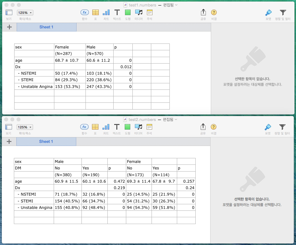
mylatex(out,size=i,caption=paste("Table ",i,". Fontsize=",i,sep=""))If you want to export your table into csv file format, you can use mycsv function.
mycsv(out,file="test.csv")
mycsv(out1,fil="test1.csv")
Following figure is a screen-shot in which test.csv and test1.csv files are opened with Numbers.
library(moonBook)
densityplot(age~sex,data=acs)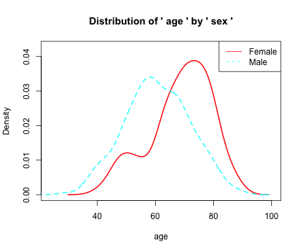
densityplot(age~Dx,data=acs)
require(survival)
data(colon)
out1=glm(status~sex+age+rx+obstruct+node4,data=colon)
out2=glm(status~rx+node4,data=colon)
ORplot(out1,type=2,show.CI=TRUE,xlab="This is xlab",main="Odds Ratio")
ORplot(out2,type=1)
ORplot(out1,type=1,show.CI=TRUE,col=c("blue","red"))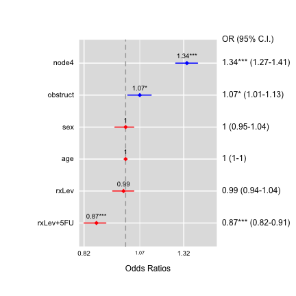
ORplot(out1,type=4,show.CI=TRUE,sig.level=0.05)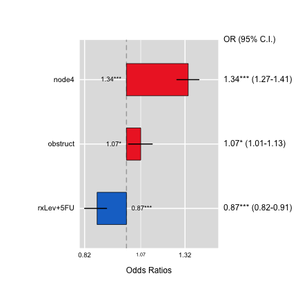
ORplot(out1,type=1,show.CI=TRUE,main="Odds Ratio",sig.level=0.05,
        pch=1,cex=2,lwd=4,col=c("red","blue"))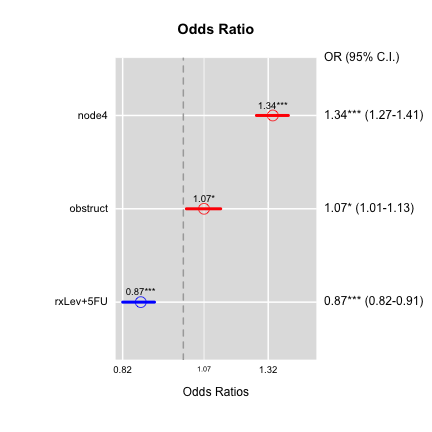
attach(colon)The following objects are masked from colon (pos = 4):
adhere, age, differ, etype, extent, id, node4, nodes,
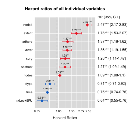
obstruct, perfor, rx, sex, status, study, surg, timecolon$TS=Surv(time,status==1)
out=mycph(TS~.,data=colon)
 mycph : perform coxph of individual expecting variables

 Call: TS ~ ., data= colon

study  was excluded : NaN
status  was excluded : infinite
out HR lcl ucl p
id 1.00 1.00 1.00 0.317
rxLev 0.98 0.84 1.14 0.786
rxLev+5FU 0.64 0.55 0.76 0.000
sex 0.97 0.85 1.10 0.610
age 1.00 0.99 1.00 0.382
obstruct 1.27 1.09 1.49 0.003
perfor 1.30 0.92 1.85 0.142
adhere 1.37 1.16 1.62 0.000
nodes 1.09 1.08 1.10 0.000
differ 1.36 1.19 1.55 0.000
extent 1.78 1.53 2.07 0.000
surg 1.28 1.11 1.47 0.001
node4 2.47 2.17 2.83 0.000
time 0.75 0.74 0.76 0.000
etype 0.81 0.71 0.92 0.001HRplot(out,type=2,show.CI=TRUE,cex=2,sig=0.05,
main="Hazard ratios of all individual variables")